Principles Involved in Farm Management Decisions

1. Law of variable proportions or Law of diminishing returns:

• It solves the problems of how much to produce ?
• It guides in the determination of optimum input to use and optimum output to produce.
• It explains the one of the basic production relationships viz., factor- product relationship.

Most Profitable level of production

(a) How much input to use.:

• Given a goal of maximizing profit, the farmer must select from all possible input levels, the one which will result in the greatest profit.
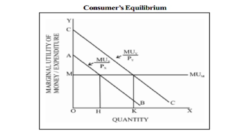
• To determine the optimum input to use, we apply two marginal concepts viz: Marginal Value Product and Marginal Factor Cost.

i) Marginal Value Product (MVP): It is the additional income received from using an additional unit of input. It is calculated by using the following equation. Marginal Value Product = Δ Total Value Product/Δ input level

MVP = ΔY. P y/Δ X

Δ = Change

Y =Output and Py = Price/unit

ii) Marginal Input Cost (MIC) or Marginal Factor Cost (MFC): It is defined as the additional cost associated with the use of an additional unit of input.

Marginal Factor Cost = Δ Total Input Cost/Δ Input level

MFC or MIC = Δ X Px/Δ X = Δ X .Px / Δ x = Px

X input Quantity Px Price per unit of input

MFC is constant and equal to the price per unit of input. This conclusion holds provided the input price does not change with the quantity of input purchased.

Decision Rules

1. If MVP is greater than MIC, additional profit can be made by using more input.
2. If MVP is less than MIC, more profit can be made by using less input.
3. Profit maximizing or optimum input level is at the point where MVP=MFC

Py (Δ Y/Δ X) = P x Δ X/ΔX

Or, Δ Y/Δ X = Px/ P y

(b) How much output to produce (Optimum output):

• To answer this question, requires the introduction of two new marginal concepts.

i) Marginal Revenue (MR): It is defined as the additional income from selling additional unit of output. It is calculated from the following equation:

Marginal Revenue = Change in total revenue / Change in Total Physical Product

MR = Δ TR / Δ Y

MR=Δ Y.Py / Δ Y = P y

Y = output

Py = price per unit of output

Total Revenue is same as Total Value Product. MR is constant and equal to the price per unit of output.

ii) Marginal Cost (MC): It is defined as the additional cost incurred from producing an additional unit of output. It is computed from the following equation.

Marginal Cost=Change in Total Cost / Change in Total Physical Product

MC=Δ X. P x/Δ Y

X= Quantity of input

Px= Price per unit of input.

Decision Rules:

1. If Marginal Revenue is greater than Marginal Cost, additional profit can be made by producing more output.
2. If Marginal Revenue is less than Marginal Cost, more profits can be made by producing less output.
3. The profit maximizing output level is at the point where MR=MC

Δ Y. P y/Δ Y=Δ X. Px/Δ Y

Or, Δ Y/Δ X= Px/P y

2. Cost principle or minimum loss principle:

• This principle guides the producers in the minimization of losses. Costs are divided into fixed and variable costs.
• Variable costs are important in determining whether to produce or not .
• Fixed costs are important in making decisions on different practices and different amounts of production.
• In the short run, the gross returns or total revenue must cover the total variable costs (TVC).
• To state in a different way that selling price must cover the average variable cost (AVC) to continue production in the short run.

Profit or decision rules

a) short run:

1. If expected selling price is greater than minimum average total cost (ATC), profit is expected and is maximized by producing where MR = MC.
2. If expected selling price is less than minimum average total cost (ATC) but greater than minimum average variable cost (AVC), a loss is expected but the loss is less than TFC and is minimized by producing where MR = MC.
3. If expected selling price is less than minimum average variable cost (AVC), a loss is expected but can be minimized by not producing anything. The loss will be equal to TFC.

b) long run:

1. Production should continue in the long run when the expected selling price is greater than minimum average total cost (ATC).
2. Expected selling price which is less than minimum ATC result in continuous losses. In this case, the fixed assets should be sold and money invested in more profitable alternative.

3. Principle of factor substitution:

• This economic principle explains one of the basic production relationships viz., factor-factor relationship.
• It guides in the determination of least cost combination of resources.
• It helps in making a management decision of how to produce.
• The principle of factor substitution says that go on adding a resource so long as the cost of resource being added is less than the saving in cost from the resource being replaced.

Profit or Decision rules

1. If Marginal rate of substitution (MRS) is greater than price ratio (PR) costs can be reduced by using more of added resource.

ΔX 2/ ΔX1 > P X1/ P X2 increase the use of X1

2. If Marginal rate of substitution (MRS ) is less than price ratio (PR), costs can be reduced by using more replaced resource.

Δ X 2/ Δ X1 < P X1/ P X2

3. Least costs combination of resources is at the point where MRS=PR

ΔX1/ Δ X2 = PX2/ P X1

Or, ΔX2/ Δ X1 = PX1/ P X2

4. Law of equi-marginal returns:

• The equi- marginal principle provides guidelines for the rational allocation of scare resources.
• The principle says that returns from the limited resources will be maximum if each unit of the resource should be used where it brings greatest marginal returns.

Example

A farmer has Rs. 3000/- and wants to grow sugarcane, wheat and cotton. What amount of money be spent on each enterprise to get maximum profits?

• The first Rs. 500 would be allocated to sugarcane as it has the highest MVP.
• The second dose of Rs. 500 would be allocated to wheat as its MVP is higher than that of cotton and sugarcane.
• In the same way, third would be used on sugarcane, the fourth, fifth and the sixth on sugarcane, wheat and cotton respectively.
• Each successive Rs of 500 is allocated to the crop which has highest marginal value product remaining after previous allocation.
• The final allocation is Rs. 1500 on sugarcane, Rs 1000 on wheat and Rs. 500 on cotton.

Opportunity cost

• Opportunity cost is defined as the returns that are sacrificed from the next best alternative.

• Opportunity cost is also known as real cost or alternate cost.

5. Principle of product substitution:

• This principle explains the product -product relationship and helps in deciding the optimum combination of products.
• Also, this economic principal guides in making a decision of what to produce.
• It is economical to substitute one product for another product, if the decrease in returns from the product being replaced is less than the increase in returns from the product being added.
• The principle of product substitution says that we should go on increasing the output of a product so long as decrease in the returns from the product being replaced is less than the increase in the returns from the product being added.

Profit rules or decision rules

• If MRS < PR, profits can be increased by producing more of added product.

MRSY1, Y2= Δ Y2/Δ Y1 < PY1/PY2, increase Y1

If MRS > PR, profits can be increased by producing more of replaced product.

MRSY1, Y2= Δ Y2/Δ Y1 < PY1/PY2, increase Y2

Optimum combination of products is when MRS= PR

i.e. Δ Y2/Δ Y1 = PY1/PY2 or,

.Δ Y1/Δ Y2 = PY2/PY1

6. Principle of comparative advantage:

• In economics, comparative advantage refers to the ability of a person or nation to produce a good or service at a lower opportunity cost than another person (or nation).
• The following example illustrates the principle of comparative advantages

• Region A has greater absolute advantage in growing both wheat and groundnut than Region B because the net incomes per acre are Rs. 75 and Rs. 25 respectively which are higher than the net incomes from wheat and groundnut in Region B.
• Farmers of Region A can make more profits by growing both the crops.
• But they want to make the greatest profits and this can be done by having the largest possible acreage under wheat alone as it is the question of relative advantage.
• Similarly, farmers of Region B have relative advantage in gr owing groundnut.

7. Time comparison principle:

• Many farm decisions involve time.
• A farmer has to decide whether to purchase new farm machinery with 10 years of life or a second hand one which may have only five years of life.
• Several other decisions involving time and initial capital investment could be judiciously taken by compounding or discounting.

a) Future value of a present sum:

• The future value of money refers to the value of an investment at a specified date in the future.
• This concept assumes that investment will earn interest which is reinvested at the end of each time period to also earn interest.
• The procedure for determining the future value of present sum is called compounding.
• The formula to find the future value of present sum in given below

FV = P (1 + i)n

where,

FV = Future value;

P = the present sum,

i = the interest rate,

n = the number of years.

Example:

Assume you have invested Rs. 100 in a savings account which earns 8% interest compounded annually and would like to know the future value of this investment after 3 years.

• In the example, a present sum of Rs. 100 has a future value of Rs. 125.97 when invested at 8 per cent interest for 3 years.
• Interest is compounded when accumulated interest also earns future interest.

b) Present value of future sum:

• Present value of future sum refers to the current value of sum of money to be received in the future.
• The procedure to find the present value of future sum is called discounting.
• The equation for finding the present value of future sum is

PV = FV/ (1+ i)n

where,

PV = Present value

FV = Future sum

i = rate of interest

n = number of years.

Examples

Example: A farmer wants to purchase a tractor. The alternatives are,

1. Purchase a new tractor for Rs. 25000/- that will last 10 years.
2. Purchase an old tractor for Rs. 15000/- and replace it after 5 years with another old tractor worth Rs. 15000/-. This means that he shall have to invest Rs. 15000/- now and lay aside an amount which will become Rs. 15000/- within 5 years to replace the old tractor.

A) Farmer with unlimited capital has the opportunity of lending the money at usual interest rate, say 5%.

PV= 15000/(1+0.05)5 = Rs. 11,760

His comparison is Rs. 25000/- for new tractor and Rs. 15000/- plus Rs.11,760/- (Rs. 26760/-) for old tractor. The new tractor is profitable for the farmer with unlimited capital.

B) Farmer with limited capital has an opportunity of investing money in poultry and can make a return of 15 % within the year. His discounting rate will be 15% i.e., opportunity cost of not using money in bank and investing in poultry.

PV= 15000/(1+0.15)5

= Rs. 7,455

His comparison is Rs. 25000/- for new tractor and Rs. 15000/- plus Rs. 7455/- (Rs. 22455/-) for old tractor. The old tractor is profitable for farmer with limited capital.